Temperature minimization
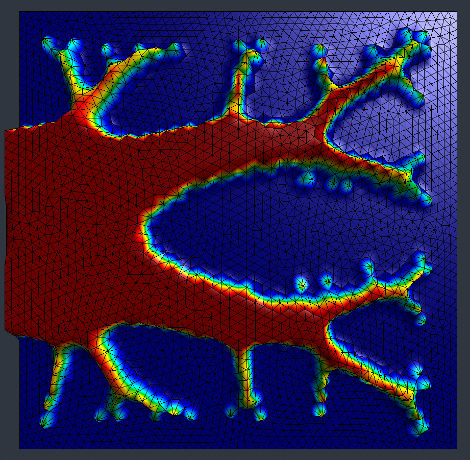
Density-based topology optimization to minimize average temperature.
Introduction
This example demonstrates density-based topology optimization using the SIMP (Solid Isotropic Material with Penalization) method. The goal is to find an optimal material distribution that minimizes the average temperature in a domain heated by a uniform source.
The optimization problem reads:
subject to the state equation (a Poisson problem with SIMP-interpolated conductivity):
where the conductivity is interpolated as .
Setup
Parameters
static constexpr int Gamma0 = 1, GammaD = 2;

static constexpr double ell   = 4;       // Lagrange multiplier
static constexpr double mu    = 0.2;     // Step size
static constexpr double gmin  = 0.0001;  // Minimum conductivity
static constexpr double gmax  = 1;       // Maximum conductivity
static constexpr double alpha = 0.05;    // Regularization parameter
static constexpr size_t maxIterations = 5000;
Mesh and Initial Density
The mesh is loaded and optimized with MMG::
MMG::Mesh Omega;
Omega.load(meshFile, IO::FileFormat::MFEM);
MMG::Optimizer().setHMax(0.005).setHMin(0.001).optimize(Omega);

P1 vh(Omega);
P1 ph(Omega);

GridFunction gamma(ph);
gamma = 0.9;  // Initial density: nearly full material
Optimization Loop
Each iteration consists of three PDE solves:
Step 1 — State Equation
The temperature field is the solution of a Poisson problem with SIMP-interpolated conductivity :
TrialFunction u(vh);
TestFunction  v(vh);
Problem poisson(u, v);
poisson = Integral((gmin + (gmax - gmin) * Pow(gamma, 3)) * Grad(u), Grad(v))
        - Integral(f * v)
        + DirichletBC(u, RealFunction(0.0)).on(GammaD);
Solver::SparseLU(poisson).solve();
Step 2 — Adjoint Equation
The adjoint problem is similar to the state equation but with a different right-hand side arising from the derivative of the objective:
TrialFunction p(vh);
TestFunction  q(vh);
Problem adjoint(p, q);
adjoint = Integral((gmin + (gmax - gmin) * Pow(gamma, 3)) * Grad(p), Grad(q))
        + Integral(RealFunction(1.0 / vol), q)
        + DirichletBC(p, RealFunction(0.0)).on(GammaD);
Solver::SparseLU(adjoint).solve();
Step 3 — Gradient and Update
The topological gradient is smoothed via a Hilbert extension-regularization solve. The density is then updated and projected to :
TrialFunction g(vh);
TestFunction  w(vh);
Problem hilbert(g, w);
hilbert = Integral(alpha * Grad(g), Grad(w))
        + Integral(g, w)
        - Integral(
            ell + 3 * (gmax - gmin) * Pow(gamma, 2)
                  Dot(Grad(u.getSolution()), Grad(p.getSolution())), w)
        + DirichletBC(g, RealFunction(0.0)).on(GammaD);
Solver::SparseLU(hilbert).solve();

GridFunction step(ph);
step = mu * g.getSolution();
gamma -= step;
gamma = Min(1.0, Max(0.0, gamma));
Full Source Code
The complete source code is:
See Also
- Poisson equation — The underlying PDE
- Shape optimization — Boundary-variation approach
- Gallery