Solving the elasticity equation
Showcases the resolution of the elasticity system.
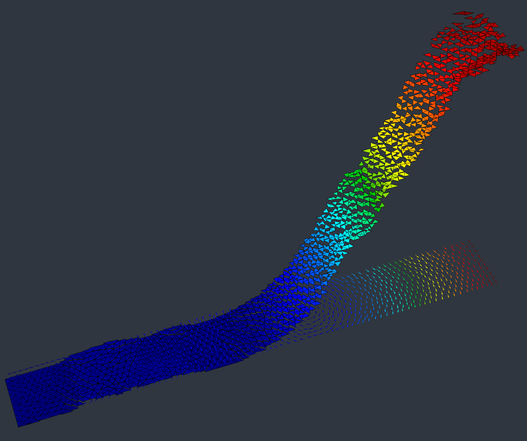
In this example we will seek to solve the linearized elasticity system. Most of the reference material in the introduction is taken from [1].
Introduction
In the elasticity setting, we are most typically interested in characterizing the elastic displacement of a mechanical structure , which in the mathematical setting is most usually defined as a bounded, Lipschitz domain, whose boundary is decomposed into three disjoint pieces: . Each piece of the boundary has the following semantic meanings:
- on the segment is where the structure is "fixed" or "attached", which is to say that the structure cannot be displaced or moved
- on the segment is where the traction loads are applied
- the remaining segment corresponds to a traction-free boundary; this is the region where the shape is free to move about
Additionally, can be subjected to body forces . In general, this framework gives rise to the linearized elasticity system:
where is known as the stress tensor of the displacement field . Furthermore, this stress tensor is related to the strain tensor
via Hooke's law
where for any in the set of symmetric matrices,
Here is the identity matrix, and , are the Lamé parameters of the constituent material, satisfying and .
Weak Formulation
As with the Poisson example, we work with the variational formulation. We seek to solve:
where . This problem is well-posed by the Lax-Milgram theorem (Korn's inequality provides coercivity).
For implementation, the bilinear form can be expanded as:
Implementation
Setup
We load the mesh using Mesh::load(), define a vector-valued P1 finite element space with components (one per spatial dimension), and set the material parameters:
#include <Rodin/Solver.h>
#include <Rodin/Geometry.h>
#include <Rodin/Variational.h>
#include <Rodin/Solid.h>

using namespace Rodin;
using namespace Rodin::Geometry;
using namespace Rodin::Variational;

// Define boundary attributes
Attribute Gamma = 1, GammaD = 2, GammaN = 3, Gamma0 = 4;

// Load mesh
Mesh mesh;
mesh.load(meshFile, IO::FileFormat::MFEM);
mesh.getConnectivity().compute(1, 2);

// Vector-valued P1 space (d components)
size_t d = mesh.getSpaceDimension();
P1 fes(mesh, d);

// Lamé coefficients
const Real lambda = 0.5769, mu = 0.3846;

// Applied traction force
VectorFunction f{0, -1};
Problem Formulation
The variational problem is expressed through the Problem class. The LinearElasticityIntegral provides a convenient shorthand for the full elasticity bilinear form. BoundaryIntegral applies the traction load on boundary segment , and DirichletBC fixes the displacement on :
TrialFunction u(fes);
TestFunction  v(fes);

Problem elasticity(u, v);
elasticity = LinearElasticityIntegral(u, v)(lambda, mu)
           - BoundaryIntegral(f, v).over(GammaN)
           + DirichletBC(u, VectorFunction{0, 0}).on(GammaD);
Solving and Output
We solve with the CG solver and save the results using IO::
Solver::CG(elasticity).solve();

// Save in MFEM format
u.getSolution().save("Elasticity.gf", IO::FileFormat::MFEM);
mesh.save("Elasticity.mesh", IO::FileFormat::MFEM);
For visualization in ParaView, export using IO::
#include <Rodin/IO/XDMF.h>

IO::XDMF xdmf("Elasticity");
xdmf.grid().setMesh(mesh).add("displacement", u.getSolution());
xdmf.write();
The full source code may be found below: