Solving the Stokes equations
Couple velocity and pressure in a lid-driven cavity.
A moving lid drags a viscous fluid around a closed square cavity. The Stokes model neglects inertia, leaving a linear system in velocity and pressure. This example introduces mixed finite elements and a pressure normalization before the Navier–Stokes tutorial adds convection and time evolution.
The mathematical problem
In , solve
The velocity and pressure are coupled by momentum balance and incompressibility. The kinematic viscosity is in nondimensional units. There is no body force.
On the lid , prescribe . The other three walls have . This regularized lid reaches unit speed at its midpoint and vanishes at both corners, avoiding the discontinuous boundary data of a constant-speed lid. Reference comparisons require the same regularized boundary profile.
Only the pressure gradient enters momentum balance. The condition fixes its arbitrary additive constant.
The mixed weak formulation
With test velocity vanishing on the boundary, test pressure , and scalar test value , the equations are
The global multiplier enforces the pressure gauge. The integral constraint fixes the additive pressure constant.
1. Construct and label the cavity
A 17-by-17 vertex grid produces 512 triangles on the unit square. Boundary edges on the top are labeled lid; the remaining exterior edges are walls.
  constexpr size_t nodes = 17;
  constexpr Attribute lid = 2;
  constexpr Attribute walls = 3;
  constexpr Real boundaryTolerance = 1e-12; // Coordinate tolerance on this unit grid.
  Mesh mesh = Mesh().UniformGrid(Polytope::Type::Triangle, {nodes, nodes});
  mesh.scale(1.0 / (nodes - 1));
  mesh.getConnectivity().compute(1, 2);
  for (auto edge = mesh.getFace(); !edge.end(); ++edge)
  {
    if (!edge->isBoundary())
      continue;
    bool onTop = true;
    for (auto vertex = edge->getVertex(); !vertex.end(); ++vertex)
      onTop = onTop && std::abs(vertex->getCoordinates().y() - 1) < boundaryTolerance;
    mesh.setAttribute({1, edge->getIndex()}, onTop ? lid : walls);
  }
2. Choose compatible spaces
Quadratic continuous velocity and linear continuous pressure form the Taylor–Hood pair. Using equal-order spaces without a suitable stabilization would be a different discretization with a different stability question. P0g supplies the single global pressure-mean multiplier.
  H1 velocitySpace(std::integral_constant<size_t, 2>{}, mesh, 2);
  H1 pressureSpace(std::integral_constant<size_t, 1>{}, mesh);
  P0g meanSpace(mesh);
  TrialFunction u(velocitySpace);
  TrialFunction p(pressureSpace);
  TrialFunction multiplier(meanSpace);
  TestFunction v(velocitySpace);
  TestFunction q(pressureSpace);
  TestFunction meanTest(meanSpace);
  constexpr Real viscosity = 1;
  VectorFunction lidVelocity{16 * Pow(F::x, 2) * Pow(1 - F::x, 2), Zero()};
  Problem stokes(u, p, multiplier, v, q, meanTest);
  stokes = viscosity * Integral(Jacobian(u), Jacobian(v)) - Integral(p, Div(v)) +
    Integral(Div(u), q) + Integral(multiplier, q) + Integral(p, meanTest) +
    DirichletBC(u, lidVelocity).on(lid) + DirichletBC(u, Zero(2)).on(walls);
The Jacobian inner product is the componentwise velocity-gradient term. The pressure term couples to the divergence of the test velocity, while the continuity equation couples the trial velocity to the pressure test function. The lid profile is interpolated into the quadratic velocity trace space.
3. Solve and inspect the circulation
The mixed formulation gives an indefinite saddle-point system. Sparse LU is adequate for this small demonstration; larger mixed problems call for suitable block preconditioning. Solver success is checked and the algebraic residual is reported before inspecting the exported fields.
  Solver::SparseLU solver(stokes);
  solver.solve();
  if (!solver.success())
    return EXIT_FAILURE;
  const auto& system = stokes.getLinearSystem();
  const Real residual =
    (system.getOperator() * system.getSolution() - system.getVector()).norm();
  std::cout << "Algebraic residual: " << residual << std::endl;
  IO::XDMF xdmf("Stokes");
  xdmf.grid()
    .setMesh(mesh)
    .add("velocity", u.getSolution())
    .add("pressure", p.getSolution());
  xdmf.write().flush();
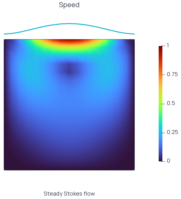
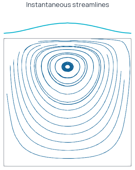
Open Stokes.xdmf, color by the magnitude of velocity, and use ParaView's Stream Tracer** to inspect the circulation. Pressure is exported separately as pressure. ParaView integrates the displayed streamlines through the exported velocity field.
Incompressibility is imposed in the pressure test space. Algebraic residuals and mesh refinement assess the numerical solution.
Complete program
See Stokes.cpp, the transient cavity example, and the solver guide.