Temperature minimization
Assemble a state, adjoint and regularized density update for heat conduction.
Domain, design and objective
On the unit square, the material density controls the conductivity
The positive lower bound keeps the state equation elliptic at zero density. With unit heat source, the temperature satisfies
The objective combines mean temperature and material usage.
Material usage is penalized with a fixed weight. The algorithm uses projected regularized gradient steps.
Discrete setup
Parameters
The state, adjoint and density use scalar continuous P1 spaces. The initial density is 0.9, the step coefficient is and the gradient regularization coefficient is . The default iteration budget is 5,000.
Mesh and sink boundary
A 32-by-32 vertex grid gives 1,024 vertices and 1,922 triangles. Boundary edges are selected as heat sinks when at least one endpoint is on the left boundary and within 0.1 of its midpoint. This endpoint-based rule defines the actual mesh-aligned sink interval.
  constexpr size_t n = 32;
  constexpr Geometry::Polytope::Type g = Geometry::Polytope::Type::Triangle;

  Alert::Info() << "Generating uniform grid..." << Alert::Raise;
  Mesh mesh = Mesh<Context::Local>::UniformGrid(g, { n, n });

  mesh.getConnectivity().compute(1, 2);
  mesh.scale(1.0 / (n - 1));

  // Boundary labeling
  for (auto it = mesh.getBoundary(); it; ++it)
  {
    bool onGammaD = false;
    for (auto vit = it->getVertex(); vit; ++vit)
    {
      const auto& vertex = *vit;
      const Real x = vertex.x();
      const Real y = vertex.y();

      if (std::abs(x) < 1e-12 && y > 0.5 - radius && y < 0.5 + radius)
      {
        onGammaD = true;
        break;
      }
    }
    mesh.setAttribute(it.key(), onGammaD ? GammaD : Gamma0);
  }
State, adjoint and update
State equation
At the current density, the state equation is assembled and solved. Factorization or solution failure terminates the program.
    Problem poisson(u, v);
    poisson = Integral(a * Grad(u), Grad(v))
            - Integral(f * v)
            + DirichletBC(u, RealFunction(0.0)).on(GammaD);
    Solver::SparseLU stateSolver(poisson);
    stateSolver.solve();
    if (!stateSolver.success())
      return EXIT_FAILURE;
Adjoint and sensitivity
Using the Lagrangian convention in this program, the adjoint satisfies
It has the same homogeneous essential boundary data as the state. The objective derivative in density direction is
    Problem adjoint(p, q);
    adjoint = Integral(a * Grad(p), Grad(q))
            + Integral(RealFunction(1.0 / vol), q)
            + DirichletBC(p, RealFunction(0.0)).on(GammaD);
    Solver::SparseLU adjointSolver(adjoint);
    adjointSolver.solve();
    if (!adjointSolver.success())
      return EXIT_FAILURE;
Regularized gradient
The derivative density is represented through
Zero gradient values on the sink keep the design's sink-boundary nodal values fixed during these updates. The coefficient convention gives a smoothing length .
    Problem hilbert(gfun, w);
    hilbert = Integral(alpha * Grad(gfun), Grad(w))
            + Integral(gfun, w)
            - Integral(
                ell
                + 3 * (gmax - gmin) * Pow(gamma, 2)
                  * Dot(Grad(u.getSolution()), Grad(p.getSolution())),
                w)
            + DirichletBC(gfun, RealFunction(0.0)).on(GammaD);
    Solver::SparseLU gradientSolver(hilbert);
    gradientSolver.solve();
    if (!gradientSolver.success())
      return EXIT_FAILURE;
Project the density
The update is . The current state, adjoint, gradient and density are exported together before the density changes, so a snapshot represents one consistent iterate.
    step = mu * gfun.getSolution();

    // Snapshot the state, adjoint and descent computed for this same density.
    xdmf.write(Real(i)).flush();
    gamma -= step;
    gamma = Min(1.0, Max(0.0, gamma));
The fixed step and fixed iteration budget define this demonstration. Assess a run through its objective, material usage and density fields. Objective-controlled step selection and an optimality stopping test are additional algorithm choices.
Inspect the results
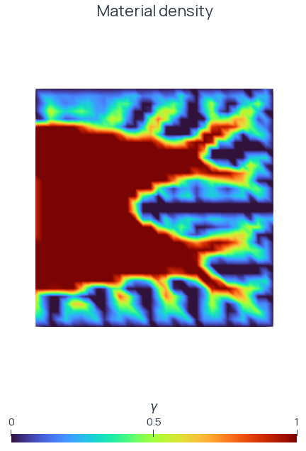
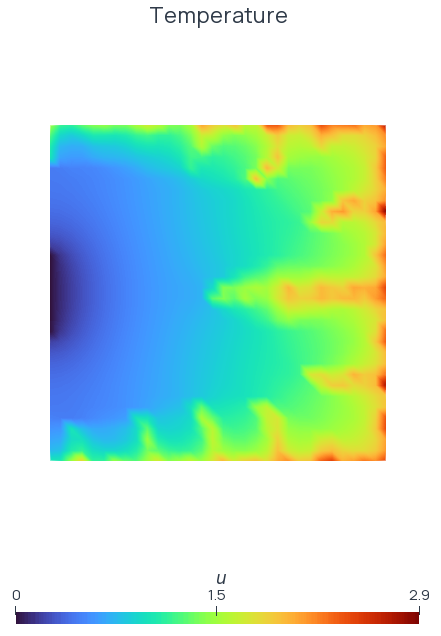
In the checked 5,000-state run, the objective decreased from approximately 4.47838 to 3.16329, with no increases in the recorded history. Material usage decreased from 0.9 to approximately 0.53165. Each state, adjoint and gradient solve succeeded. These observations describe the fixed-step run.
TemperatureMinimization.csv records mean temperature, material usage and their weighted objective. The XDMF output contains temperature u, adjoint p**, regularized gradient g, density gamma and update step. Open TemperatureMinimization.xdmf in ParaView and select Apply.
Build and run
Build TemperatureMinimization. The executable generates its mesh, so no resource file is required. Run it in a scratch directory; an optional positive integer argument selects the iteration budget. Omitting it runs 5,000 updates. The program checks each sparse solve and each recorded objective for failure.
Complete source code contains the boundary selection and numerical update.