Solving the Poisson equation
Resolution of the Poisson equation using Rodin.
Introduction
The Poisson equation is the "Hello World!" of the finite element method. It arises in many physical contexts: heat conduction, electrostatics, gravitational potential, and membrane deflection. In this example we solve:
where is the unit square, is a constant source term, and we impose homogeneous Dirichlet boundary conditions on the entire boundary .
Weak Formulation
To solve this PDE numerically with the finite element method, we first derive its weak (variational) formulation. Multiplying by a test function and integrating by parts:
The boundary term vanishes because on .
Includes and Namespaces
We need the following Rodin modules:
- Geometry — for the Mesh class
- Variational — for P1, TrialFunction, TestFunction, and the Problem class
- Solver — for the CG iterative solver
- IO::
XDMF — for exporting results to ParaView
#include <Rodin/Solver.h>
#include <Rodin/Geometry.h>
#include <Rodin/Variational.h>
#include <Rodin/IO/XDMF.h>

using namespace Rodin;
using namespace Rodin::Solver;
using namespace Rodin::Geometry;
using namespace Rodin::Variational;
Creating the Mesh
We create a triangular mesh on the unit square using Mesh::UniformGrid() with a grid. We also compute the face-to-cell connectivity (dimension 1 to dimension 2) via Connectivity::compute(), which is needed to identify boundary faces for imposing Dirichlet conditions:
Mesh mesh;
mesh = mesh.UniformGrid(Polytope::Type::Triangle, { 16, 16 });
mesh.getConnectivity().compute(1, 2);
This creates a mesh with triangular cells and vertices.
Finite Element Space
We define a P1 (piecewise linear, continuous) finite element space on the mesh, and create the TrialFunction and TestFunction:
P1 vh(mesh);

TrialFunction u(vh);
TestFunction  v(vh);
The trial function represents the unknown solution, and the test function is used to express the weak formulation. After solving, the computed solution coefficients are accessible via u.getSolution().
Problem Formulation
The variational problem is assembled using Rodin's form language through the Problem class. The code closely mirrors the mathematical notation:
RealFunction f = 1;

Problem poisson(u, v);
poisson = Integral(Grad(u), Grad(v))
        - Integral(f, v)
        + DirichletBC(u, Zero());
Here:
Integral(Grad(u), Grad(v))represents the bilinear formIntegral(f, v)represents the linear formDirichletBC(u, Zero())enforces on the entire boundary
Solving
We solve the problem using the CG (Conjugate Gradient) iterative solver, which is well-suited for symmetric positive definite systems like the one arising from the Poisson equation:
CG(poisson).solve();
Alternative solvers include SparseLU (direct) and GMRES (for non-symmetric systems).
Exporting to XDMF
After solving, we export the mesh and solution using the IO::
IO::XDMF xdmf("Poisson");
xdmf.grid().setMesh(mesh).add("u", u.getSolution());
xdmf.write();
This produces:
Poisson.xdmf— the XML metadata file (open this in ParaView)Poisson.*.h5— HDF5 data files containing the mesh and solution
To visualize in ParaView:
- Open
Poisson.xdmf - Click Apply
- Select "u" from the field dropdown
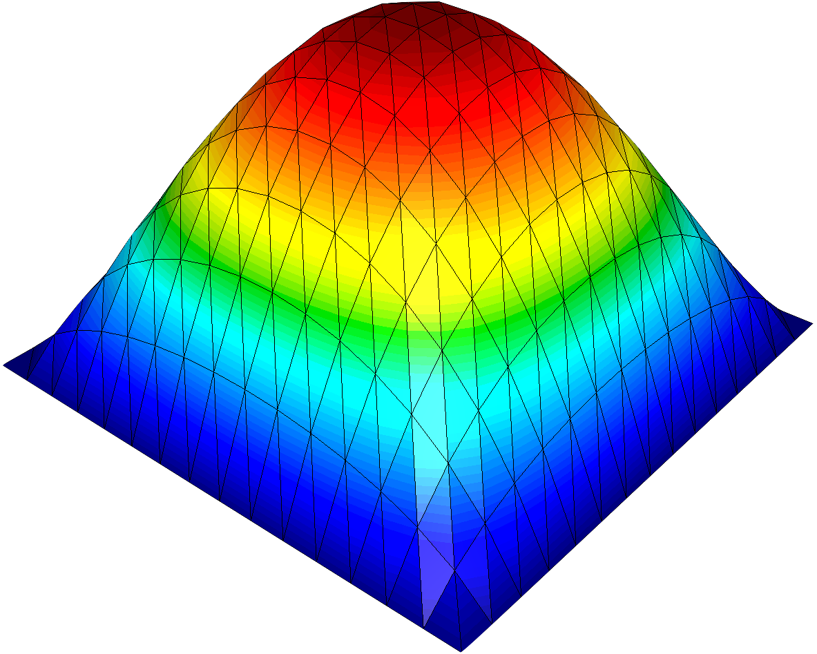
- Use the Warp By Scalar filter for a 3D surface plot
Full Source Code
The complete source code is: