Evaluating interface traces
Inspect two cell values, their jump and their arithmetic average.
A discontinuous field
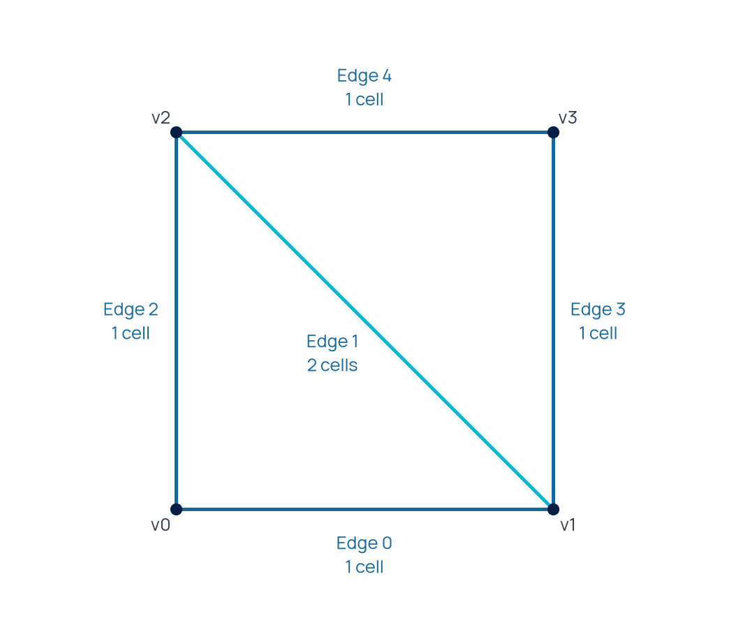
A square split into two triangles has one interior facet. A piecewise constant field takes value one in region one and value three in region two. This small example makes side selection explicit before facet terms are used in a variational formulation.
  Mesh mesh = Mesh().UniformGrid(Polytope::Type::Triangle, {2, 2});
  mesh.getConnectivity().compute(1, 2);
  mesh.setAttribute({2, 0}, 1);
  mesh.setAttribute({2, 1}, 2);
  P0 vh(mesh);
  GridFunction field(vh);
  field = RealFunction([](const Point& point) {
    return point.getPolytope().getAttribute() == 1 ? 1.0 : 3.0;
  });
The mesh is the same two-triangle topology used in the connectivity tutorial.
Select and combine traces
The facet midpoint is mapped back into each incident cell. Evaluating the field on those two cell points obtains the one-sided values explicitly. Jump subtracts the two incident-cell values in the library's incidence order. Average forms their arithmetic mean.
  const auto jump = Jump(field);
  const auto average = Average(field);

  constexpr Real tolerance = 1e-12;
  bool valid = true;
  size_t interfaces = 0;
  std::ofstream samples("InterfaceTraces.csv");
  samples << "x,y,first,second,jump,average\n";
  for (auto face = mesh.getInterface(); !face.end(); ++face)
  {
    const Point point(*face, Math::SpatialPoint{0.5});
    const auto firstCell = mesh.getCell(0);
    const auto secondCell = mesh.getCell(1);
    Math::SpatialPoint firstReference, secondReference;
    firstCell->getTransformation().inverse(
      firstReference, point.getPhysicalCoordinates());
    secondCell->getTransformation().inverse(
      secondReference, point.getPhysicalCoordinates());
    const Real first = field(Point(*firstCell, firstReference));
    const Real second = field(Point(*secondCell, secondReference));
    const Real value = jump(point);
    const Real mean = average(point);
    samples << point.x() << ',' << point.y() << ',' << first << ',' << second << ','
            << value << ',' << mean << '\n';
    std::cout << "Traces: " << first << ", " << second << "; jump: " << value
              << "; average: " << mean << std::endl;
    valid = valid && std::abs(first - 1) < tolerance &&
      std::abs(second - 3) < tolerance && std::abs(std::abs(value) - 2) < tolerance &&
      std::abs(mean - 2) < tolerance;
    ++interfaces;
  }
| Quantity | Expected value |
|---|---|
| Trace from region one | 1 |
| Trace from region two | 3 |
| Absolute jump | 2 |
| Arithmetic average | 2 |
The sign of a jump follows the incidence ordering. A flux formula must use the matching normal convention. Attribute-based trace selection gives an explicit side when modeling a material interface.
Run and inspect
Build the InterfaceTraces target. The program evaluates the midpoint of the interior facet, prints the four values and exports InterfaceTraces.csv. It checks the table above with tolerance and returns EXIT_FAILURE if a check fails.
The complete program is available in InterfaceTraces.cpp.