Computing arrival times with fast marching
Propagate from one exact seed, compare with an analytic distance and check refinement.
Arrival time and speed
A front propagates through the unit square with positive speed . The arrival time satisfies
For constant speed , the exact solution is
Unit speed produces distance; doubling the speed halves every arrival time. This provides a direct check of the speed convention used by FMM.
Choose an exact seed
The program uses triangular grids with 16, 32 and 64 intervals per axis. Each count is even, so the center is a mesh vertex at every refinement. Seeding a neighborhood around the center would prescribe zero time on a larger source set and change the reference problem.
      const size_t n = intervals + 1;
      const Real h = Real(1) / intervals;
      auto mesh = LocalMesh::UniformGrid(Polytope::Type::Triangle, {n, n});
      mesh.scale(h);
      mesh.getConnectivity().compute(2, 0);
      mesh.getConnectivity().compute(0, 2);
      mesh.getConnectivity().compute(0, 0);
Vertex-to-cell incidence supplies the local simplicial stencils. Vertex-to-vertex incidence supplies neighboring trial vertices. Both are prepared before seeding and propagation.
Propagate the front
A scalar continuous field stores nodal arrival times. The source contains exactly one vertex. seed() sets its value to zero and initializes neighboring trial values; solve() repeatedly accepts the smallest trial arrival time and updates its neighbors.
      P1 space(mesh);
      GridFunction arrival(space);
      IndexVector seeds;
      for (auto vertex = mesh.getVertex(); vertex; ++vertex)
      {
        const auto& x = vertex->getCoordinates();
        if (x(0) == Real(0.5) && x(1) == Real(0.5))
          seeds.push_back(vertex->getIndex());
      }
      if (seeds.size() != 1)
        return EXIT_FAILURE;
      const auto speed = [propagationSpeed](const Point&) { return propagationSpeed; };
      Eikonal::FMM marching(arrival, speed);
      marching.seed(seeds).solve();
The callable returns propagation speed in distance per unit time. Supply finite, strictly positive values. Its reciprocal is the local slowness. This example uses constant speeds 1 and 2, with identical grids and seeds.
Compare with the analytic field
For the nodal set , the program records
These are nodal error measures. The arithmetic mean is independent of cell areas and differs from an integrated error norm.
      Real maximum = 0, mean = 0;
      for (auto vertex = mesh.getVertex(); vertex; ++vertex)
      {
        const auto& x = vertex->getCoordinates();
        const auto& dofs = space.getDOFs(0, vertex->getIndex());
        const Real computed = arrival.getData()(dofs[0]);
        const Real exact =
          std::hypot(x(0) - Real(0.5), x(1) - Real(0.5)) / propagationSpeed;
        const Real error = std::abs(computed - exact);
        valid = valid && std::isfinite(computed) && computed >= 0;
        maximum = std::max(maximum, error);
        mean += error;
      }
      mean /= mesh.getVertexCount();
      // A deliberately loose O(h) regression envelope on this mesh sequence.
      // Measured errors, rather than this bound, characterize the observed rate.
      valid =
        valid && maximum < previousError && maximum <= Real(2) * h / propagationSpeed;
      previousError = maximum;
      errors << intervals << ',' << propagationSpeed << ',' << maximum << ',' << mean
             << '\n';
The checked local results for unit speed are:
| Intervals per axis | Vertices | Maximum nodal error | Mean nodal error |
|---|---|---|---|
| 16 | 289 | ||
| 32 | 1089 | ||
| 64 | 4225 |
Both errors decrease under refinement. With speed 2, every tabulated error is halved to printed precision. The point-source solution has a singular gradient at the center; this sequence supplies measured convergence for this setup, without assuming the interpolation order of a smooth field.
The executable requires finite nonnegative arrival times, a unique source, strictly decreasing maximum errors and the loose regression envelope . That envelope is a check for this example's grids. Assess other geometries and variable-speed fields against their own reference solutions or refinement studies.
Build and inspect
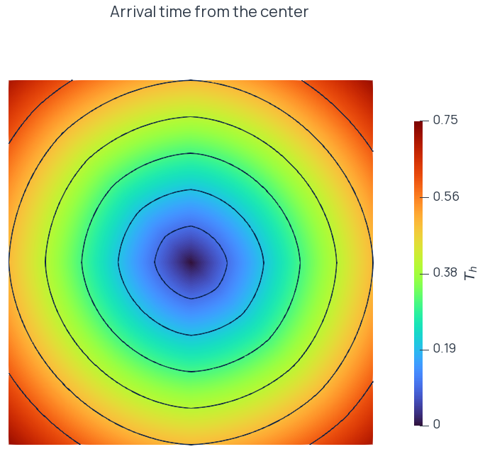
Build the Eikonal_FMM target and run it in a scratch directory. It needs no input mesh. FMMErrors.csv contains all six refinement/speed results. FMMArrival.xdmf and its HDF5 companions contain the finest unit-speed computed field arrival and interpolated analytic nodal field reference. Open the XDMF in ParaView and select Contour on arrival to inspect the advancing fronts.
Complete program
The complete program is available in FMM.cpp.
Distance fields in applications
A zero-time vertex set defines an unsigned arrival-time problem. Signed level-set reconstruction additionally needs an inside/outside convention. The shape optimization guide describes transport and redistancing; Adapting and fitting an implicit interface shows how an analytic signed distance can drive mesh-interface fitting.