Adapting and fitting an implicit interface
Prepare a graded background with MMG, classify a circle, and fit its interface with SWIFT.
Geometry and workflow
Consider a circle of radius centered at inside the unit square. Its signed distance and gradient are
The negative phase is the disk. The gradient is undefined at the center; the callable returns zero there, away from the interface being fitted.
A background mesh must provide enough resolution near the circle and a set of facets that can represent its boundary. The example uses three stages:
- MMG changes the background mesh according to a positive size field.
- MinSTCut assigns inside/outside cell labels and marks separating facets.
- SWIFT displaces those facets towards the circle while holding the outer square fixed and checking its sampled mesh-quality budget.
This sequence is also used in the Kelvin ball application. Here the analytic target isolates geometry fitting from PDE solves, level-set transport and field transfer. The size-field tutorial supplies the remeshing background; SWIFT explains the fitting model.
Prepare the background
The initial grid has 13 vertices per axis and 288 triangles. Let be its spacing. The target edge size is
with , and in unit-square coordinates. Thus the requested mesh is fine near the circle and coarser away from it. These are chosen mesh-design parameters. The exponential is the weight supplied by Loss.
    {
      P1 sizeSpace(mesh);
      MMG::RealGridFunction size(sizeSpace);
      const SWIFT::Loss band(BandWidth);
      size = [&](const Point& point) {
        return FarSize - (FarSize - NearSize) * band.getWeight(phi(point));
      };
      MMG::Adapt().setHMin(NearSize).setHMax(FarSize).setGradation(Gradation).adapt(
        mesh, size);
    }
    // All fields below are constructed on the new mesh.
MMG receives scalar nodal sizes, lower/upper size limits and a gradation parameter of . The four box corners are marked before adaptation. The size field is scoped to that call. All subsequent spaces and solvers are constructed on the adapted topology.
Label the phases
On each adapted cell , define the local scale and approximate the cell average
MinSTCut combines fidelity to these averages with a separating-facet cost. The facet weight is on an interior facet. Second-order quadrature approximates the nonpolynomial phase average. The phase width and smoothing coefficient are classification choices.
    constexpr Real PhaseWidth = Real(1.25), Smoothing = Real(0.01);
    constexpr size_t ClassificationOrder = 2;
    MinSTCut classifier(static_cast<const LocalMesh&>(mesh));
    decltype(classifier)::Parameters classification;
    classification.smoothing = [&](const Polytope& face) {
      const auto& cells = mesh.getConnectivity().getIncidence({1, 2}, face.getIndex());
      Real localSize = std::sqrt(mesh.getPolytope(2, cells[0])->getMeasure());
      for (const Index cell : cells)
      {
        localSize =
          std::min(localSize, std::sqrt(mesh.getPolytope(2, cell)->getMeasure()));
      }
      return Smoothing * localSize;
    };
    classifier.setParameters(classification);
    const auto labels = classifier.classify([&](const Polytope& cell) {
      const Real localSize = std::sqrt(cell.getMeasure());
      const auto& formula =
        QF::QuadratureFormula::get(ClassificationOrder, cell.getGeometry());
      const auto& quadrature = cell.getQuadrature(formula);
      Real moment = 0;
      for (size_t q = 0; q < quadrature.getSize(); ++q)
      {
        const auto& point = quadrature.getPoint(q);
        moment += formula.getWeight(q) * point.getDistortion() *
          std::tanh(phi(point) / (PhaseWidth * localSize));
      }
      return moment / cell.getMeasure();
    });
    for (const Index cell : labels.inside)
      mesh.setAttribute({2, cell}, Inside);
    for (const Index cell : labels.outside)
      mesh.setAttribute({2, cell}, Outside);
    for (const Index face : labels.cut)
      mesh.setAttribute({1, face}, Interface);
    for (auto face = mesh.getFace(); face; ++face)
    {
      if (mesh.getConnectivity().getIncidence({1, 2}, face->getIndex()).size() == 1)
        mesh.setAttribute({1, face->getIndex()}, Boundary);
    }
Cells receive attributes 1 and 2, separating edges receive attribute 10, and exterior edges receive attribute 20. Classification changes labels. The resulting polygonal interface follows existing mesh edges.
Fit the marked interface
The local Adapt workflow owns a vector-valued continuous displacement space. Its increment is zero on the outer square. The analytic distance and gradient supply the target throughout the solve.
    RealFunction phi([](const Point& point) {
      return std::hypot(point.x() - Real(0.5), point.y() - Real(0.5)) - Radius;
    });
    VectorFunction gradient(2, [](const Point& point) {
      Math::SpatialVector<Real> radial(2);
      radial(0) = point.x() - Real(0.5);
      radial(1) = point.y() - Real(0.5);
      const Real length = radial.norm();
      if (length == 0)
        return Math::SpatialVector<Real>::Zero(2);
      return Math::SpatialVector<Real>(radial / length);
    });
    SWIFT::Adapt fitting(mesh);
    SWIFT::Parameters parameters;
    parameters.model.h = NearSize;
    parameters.linear.solver = SWIFT::Parameters::LinearSolver::SparseLU;
    parameters.convergence.tolerance.geometric = GeometricTolerance;
    fitting.setParameters(parameters).setInterfaceAttribute(Interface);
    fitting.getProblem() +=
      DirichletBC(fitting.getTrialFunction(), VectorFunction(Real(0), Real(0)))
        .on(Boundary);
    std::ofstream history("BackgroundFitting.csv");
    history << std::setprecision(17) << "iteration,energy,geometric_error,min_j,max_q\n";
    fitting.getProblem().setMonitor([&](const SWIFT::Report& report) {
      history << report.iterations << ',' << report.energy << ',' << report.geometricSup
              << ',' << report.minJ << ',' << report.maxQRel << '\n';
    });
    const auto report = fitting.execute(phi, gradient);
Here model.h is fixed at the requested near-interface size, . It scales the fitting model throughout this solve. An explicit geometric tolerance of replaces the automatic stopping target. The local SparseLU backend is selected explicitly. Other model and work-budget settings retain their defaults.
execute() applies the accepted displacement to the mesh when the sampled quality budget is satisfied. A quality-valid best-effort result may still miss the geometric tolerance; this tutorial additionally requires geometricTargetReached before returning success. The fitting stage preserves the adapted connectivity and cell labels.
Inspect the result
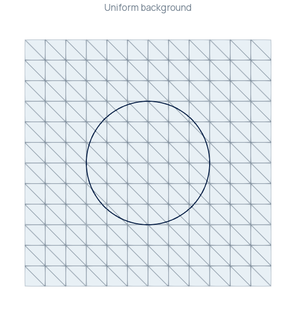
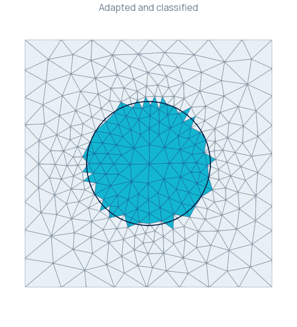
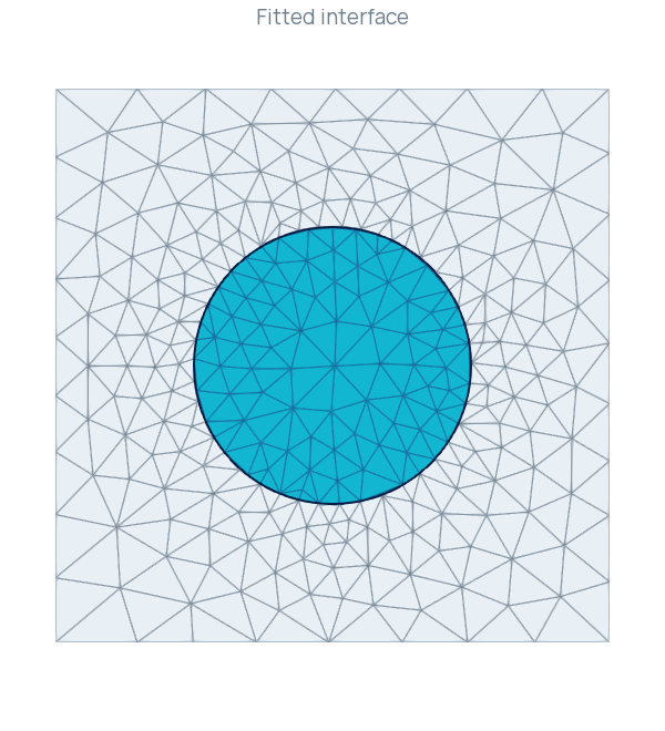
These are the actual meshes written by the program. Edges remain visible to show where fitting compresses elements. The navy circle supplies the same analytic reference in every panel.
The checked local run produced the following measurements:
| Quantity | Result |
|---|---|
| Uniform background | 169 vertices, 288 triangles |
| Adapted background | 288 vertices, 540 triangles |
| Classified interface | 49 edges |
| Accepted fitting steps | 5 |
| Maximum radial error on the complete polygonal interface | |
| Minimum relative Jacobian | |
| Maximum relative distortion | |
| Outer-boundary displacement |
For a straight interface segment, the radial distance is largest at an endpoint and smallest at the orthogonal projection of the center, clamped to that segment. Evaluating these locations gives an independent maximum radial error on every complete segment. It agrees with the solver's sampled maximum to floating-point precision in this run. This checks the distance from the reconstructed interface to the circle; a two-sided Hausdorff calculation would also examine distances from the circle back to the polygon.
Every triangle has a positive signed Jacobian, the square retains unit area, and fitting leaves its vertex and cell counts unchanged. The relative Jacobian and distortion values also show substantial local compression. Passing the configured budget permits this deformation. A subsequent PDE application should assess element conditioning and its own approximation error before choosing these mesh parameters.
Build, run and visualize
Build and execute the SWIFT_BackgroundFitting target in a scratch directory.
cmake --build build --target SWIFT_BackgroundFitting
mkdir -p results/background-fitting
cd results/background-fitting
../../build/examples/Adaptation/SWIFT/SWIFT_BackgroundFitting
BackgroundFitting.xdmf contains the named blocks uniform, classified and fitted. Keep its HDF5 companions alongside it. In ParaView, use Extract Block to select a stage, then Surface With Edges. On the last two blocks, threshold the cell array Attribute at 1 to show the disk. BackgroundFitting.csv records accepted-step diagnostics; the final monitor notification may repeat the last accepted step.
Complete program
The complete program is available in BackgroundFitting.cpp.
Continue
The shared SWIFT_ReconstructionP1, SWIFT_ReconstructionP2 and SWIFT_ReconstructionP3 examples extend fitting to lobed targets and curved geometry. They retain an unchanged reference mesh while evaluating the displacement at all geometry nodes. See Fitting a mesh interface with SWIFT for ownership, higher-order geometry updates and diagnostic definitions.