Constructing a distance approximation from a Poisson field
Mesh three implicit disks, solve a signed auxiliary problem and inspect its normalization error.
The geometric reference
Let contain three disks with centers and radii
| Center | Radius |
|---|---|
The largest disk touches the square at two points. The disks have disjoint interiors. Their union has signed distance
negative inside and positive outside. This analytic field supplies both the implicit geometry and a reference for the normalized output.
    RealFunction exact([](const Point& point) {
      return std::min(
        {std::hypot(point.x() - Real(0.75), point.y() - Real(0.25)) - Real(0.05),
          std::hypot(point.x() - Real(0.25), point.y() - Real(0.25)) - Real(0.25),
          std::hypot(point.x() - Real(0.75), point.y() - Real(0.75)) - Real(0.10)});
    });
Resolve and label the interface
The background has 32 vertices per axis. Its nodal interpolation approximates the signed-distance field. MMG cuts the zero level set of that interpolant and remeshes with maximum requested edge size .
    {
      P1 initialSpace(mesh);
      MMG::RealGridFunction levelSet(initialSpace);
      levelSet = exact;
      mesh = MMG::LevelSetDiscretizer()
               .split(BaseMaterial, {Inside, Outside})
               .setBoundaryReference(Interface)
               .setAngleDetection()
               .setHMax(MaximumSize)
               .discretize(levelSet);
    }
    mesh.getConnectivity().compute(1, 2);
The material split explicitly assigns inside cells attribute 3, outside cells attribute 2 and interface edges attribute 5. The field used to drive remeshing is scoped to that operation. The following solve uses a new space on the returned mesh.
In the checked run, the result has 3,852 vertices and 7,458 triangles. Its inside area is , compared with the analytic disk area . Refining the background interpolation is part of controlling this geometric discrepancy; remeshing a fixed interpolant retains its zero-set approximation.
Solve the auxiliary problem
With the mesh's inside region and its marked interface, the scalar potential satisfies
The exterior boundary portions have the homogeneous Neumann condition of the weak formulation. The force is negative inside and positive outside. The fitted interface provides the essential condition that anchors each region. The corresponding constrained stiffness matrix is symmetric positive definite.
The program constructs this problem explicitly so that CG convergence and the assembled residual can be checked before normalization. The same attributed forcing is used by SignedPoisson.
    P1 space(mesh);
    TrialFunction u(space);
    TestFunction v(space);
    Problem potential(u, v);
    potential = Integral(Grad(u), Grad(v)) + Integral(2 * v).over(Inside) - Integral(v) +
      DirichletBC(u, Zero()).on(Interface);
    Solver::CG solver(potential);
    constexpr Real LinearTolerance = Real(1e-10);
    solver.setTolerance(LinearTolerance).solve();
    if (!solver.success())
      return EXIT_FAILURE;
    const auto& system = potential.getLinearSystem();
    const Real relativeResidual =
      (system.getOperator() * system.getSolution() - system.getVector()).norm() /
      std::max(Real(1), system.getVector().norm());
    constexpr Real ResidualTolerance = Real(1e-9);
    if (!std::isfinite(relativeResidual) || relativeResidual > ResidualTolerance)
      return EXIT_FAILURE;
    const auto& poisson = u.getSolution();
    auto normalized = Distance::SpaldingTucker()(poisson);
    GridFunction reference(space);
    reference = exact;
SpaldingTucker evaluates
and interpolates it into the input space. A positive denominator preserves the sign of the potential pointwise. The expression requires a defined gradient and becomes undefined when the potential and its gradient vanish together. The executable checks the resulting nodal values for finiteness.
Inspect the approximation
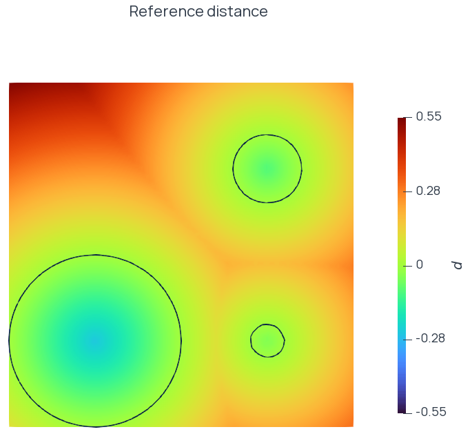
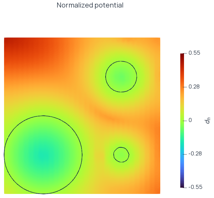
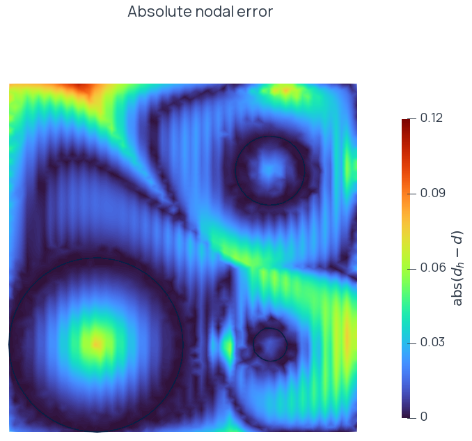
The two signed fields use the same color range, . The error range is . Dark contours show the meshed interface. Dense triangle edges are omitted to keep the scalar fields readable.
The checked local run produced:
| Quantity | Value |
|---|---|
| Maximum absolute nodal error | |
| Arithmetic mean absolute nodal error | |
| Maximum normalized value on interface vertices | |
The arithmetic mean is over mesh vertices and differs from an area-weighted error norm. The maximum occurs on the upper boundary near , where the normalized value is and the reference value is .
The normalization has an intrinsic multidimensional approximation error. For a single disk with the exact radial interior potential , the center value becomes , whereas the signed distance is . For , this gives an absolute center discrepancy of before any discretization. The three-disk computation also includes interface approximation, finite element gradients and the outer Neumann boundary. Distance accuracy is assessed through the reference comparison in addition to the linear residual.
Build and inspect the output
Build the SpaldingTucker target and run it in a scratch directory. It generates its input mesh and writes DistanceNormalization.xdmf with its HDF5 companions. The arrays are potential, normalized and reference. DistanceNormalization.csv records mesh counts, inside area, nodal errors, interface values and the relative algebraic residual.
The program requires CG success, a residual below , finite nodal fields, nonempty inside/outside regions and interface values within of zero. The recorded distance errors describe this approximation and geometry.
Complete program
The complete program is available in SpaldingTucker.cpp.
Continue
- Computing arrival times with fast marching — Arrival-time propagation and mesh refinement.
- Adapting and fitting an implicit interface — Interface fitting driven by signed distance.
- Shape and topology optimization — Level-set transport and redistancing.