Solving diffusion with discontinuous Galerkin
Assemble and validate a symmetric interior-penalty method on triangles.
Problem and discrete space
On , solve
The discontinuous space is
Each triangle owns three affine coefficients. Neighboring triangles have independent values at a shared geometric vertex. Thus a mesh with cells has unknowns.
This example assembles the cell and facet matrices explicitly using Rodin meshes, mapped quadrature and sparse algebra. The implementation is scoped to affine two-dimensional triangles. Making every local block visible connects the consistency and penalty terms to their actual matrix entries.
Interior flux and penalty
For each interior facet, order the cells as and choose outward from . Define
With facet length and , the symmetric form is
The right-hand side is
Boundary coefficients remain unknown. The boundary terms impose the data weakly. The penalty value is a fixed choice for the degree-one, shape-regular meshes studied here; other degrees or cell shapes require an appropriate penalty analysis.
Cell and facet matrices
On the reference triangle, the basis is . Its physical gradients are obtained with . Index identifies local basis function in cell .
      // Affine triangle basis: (1-r-s, r, s). Coefficients belong to cells.
      const std::array<Math::SpatialVector<Real>, 3> referenceGradients = {
        Math::SpatialVector<Real>{-1, -1}, {1, 0}, {0, 1}};
      std::vector<std::array<Math::SpatialVector<Real>, 3>> gradients(count);
      for (auto cell = mesh.getCell(); !cell.end(); ++cell)
      {
        const Point center(*cell, Math::SpatialPoint{1.0 / 3, 1.0 / 3});
        for (size_t i = 0; i < 3; ++i)
        {
          gradients[cell->getIndex()][i] =
            center.getJacobianInverse().transpose() * referenceGradients[i];
        }
      }
      Math::SparseMatrix<Real> matrix(dofs, dofs);
      Math::Vector<Real> rhs = Math::Vector<Real>::Zero(dofs);
      std::vector<Math::SparseTriplet<Real>> entries;
      const auto& cellFormula =
        QF::QuadratureFormula::get(size_t{10}, Polytope::Type::Triangle);
      for (auto cell = mesh.getCell(); !cell.end(); ++cell)
      {
        const Index k = cell->getIndex();
        for (size_t i = 0; i < 3; ++i)
        {
          for (size_t j = 0; j < 3; ++j)
          {
            entries.emplace_back(3 * k + i, 3 * k + j,
              cell->getMeasure() * gradients[k][i].dot(gradients[k][j]));
          }
        }
        PolytopeQuadrature points(*cell, cellFormula);
        for (size_t q = 0; q < points.getSize(); ++q)
        {
          const auto& p = points.getPoint(q);
          const auto& r = cellFormula.getPoint(q);
          const std::array<Real, 3> basis = {1 - r.x() - r.y(), r.x(), r.y()};
          const Real f =
            patch ? 0 : 2 * pi * pi * std::sin(pi * p.x()) * std::sin(pi * p.y());
          const Real weight = cellFormula.getWeight(q) * p.getJacobianDeterminant();
          for (size_t i = 0; i < 3; ++i)
            rhs[3 * k + i] += weight * f * basis[i];
        }
      }
An interior facet contributes a six-by-six block over both cells. A boundary facet contributes a three-by-three block and a load vector. The implementation uses the same normal and cell ordering in every jump and flux term.
      const auto& faceFormula =
        QF::QuadratureFormula::get(size_t{10}, Polytope::Type::Segment);
      for (auto face = mesh.getFace(); !face.end(); ++face)
      {
        const auto& incident =
          mesh.getConnectivity().getIncidence({1, 2}, face->getIndex());
        std::vector<Index> cells(incident.begin(), incident.end());
        const bool boundary = cells.size() == 1;
        const auto firstCell = mesh.getCell(cells[0]);
        const Point center(*firstCell, Math::SpatialPoint{1.0 / 3, 1.0 / 3});
        const Point midpoint(*face, Math::SpatialPoint{0.5});
        const auto vertices = face->getVertex();
        auto next = face->getVertex();
        ++next;
        const Math::SpatialVector<Real> tangent =
          next->getCoordinates() - vertices->getCoordinates();
        Math::SpatialVector<Real> normal{tangent.y(), -tangent.x()};
        const Real length = normal.norm();
        normal /= length;
        if (normal.dot(
              midpoint.getPhysicalCoordinates() - center.getPhysicalCoordinates()) < 0)
          normal *= -1;
        const Real sigma = penalty / length;
        PolytopeQuadrature points(*face, faceFormula);
        for (size_t q = 0; q < points.getSize(); ++q)
        {
          const auto& p = points.getPoint(q);
          const Real weight = faceFormula.getWeight(q) * p.getJacobianDeterminant();
          std::array<Real, 6> jump{};
          std::array<Real, 6> normalDerivative{};
          for (size_t side = 0; side < cells.size(); ++side)
          {
            const auto cell = mesh.getCell(cells[side]);
            Math::SpatialPoint r;
            cell->getTransformation().inverse(r, p.getPhysicalCoordinates());
            const std::array<Real, 3> basis = {1 - r.x() - r.y(), r.x(), r.y()};
            for (size_t i = 0; i < 3; ++i)
            {
              const size_t local = 3 * side + i;
              jump[local] = (side == 0 ? 1 : -1) * basis[i];
              normalDerivative[local] =
                (boundary ? 1 : 0.5) * gradients[cells[side]][i].dot(normal);
            }
          }
          const size_t localSize = 3 * cells.size();
          for (size_t i = 0; i < localSize; ++i)
          {
            const Index row = 3 * cells[i / 3] + i % 3;
            for (size_t j = 0; j < localSize; ++j)
            {
              const Index column = 3 * cells[j / 3] + j % 3;
              const Real value = -normalDerivative[j] * jump[i] -
                normalDerivative[i] * jump[j] + sigma * jump[i] * jump[j];
              entries.emplace_back(row, column, weight * value);
            }
            if (boundary)
              rhs[row] += weight * exact(p) * (-normalDerivative[i] + sigma * jump[i]);
          }
        }
      }
Degree-ten quadrature integrates the polynomial stiffness and penalty terms exactly on these affine cells. It also resolves the smooth prescribed source and error integrals used in the refinement study.
Solve and check the algebra
The assembled matrix is checked for relative symmetry. A sparse LDLT factorization checks positive pivots, solves the system and reports the relative algebraic residual. These checks concern each actual assembled system in the study.
      matrix.setFromTriplets(entries.begin(), entries.end());
      const Math::SparseMatrix<Real> transpose = matrix.transpose();
      const Real symmetry = (matrix - transpose).norm() / matrix.norm();
      Eigen::SimplicialLDLT<Math::SparseMatrix<Real>> solver;
      solver.compute(matrix);
      if (solver.info() != Eigen::Success || solver.vectorD().minCoeff() <= 0)
        return EXIT_FAILURE;
      const Math::Vector<Real> solution = solver.solve(rhs);
      if (solver.info() != Eigen::Success)
        return EXIT_FAILURE;
      const Real residual = (matrix * solution - rhs).norm() / rhs.norm();
      valid = valid && symmetry < algebraTolerance && residual < algebraTolerance;
Stability and optimal error estimates for consistent interior-penalty methods are developed by Arnold, Brezzi, Cockburn and Marini [2].
Patch test and refinement study
The first case is , with zero source and nonzero Dirichlet data. It is exactly representable in the discontinuous affine space. The measured error is and the broken-gradient error is .
The second case uses
The program refines the mesh while retaining the degree, penalty convention, source, boundary data and quadrature order.
| Intervals per axis | Unknowns | | | | —: | —: | —: | —: | | 4 | 96 | | | | 8 | 384 | | | | 16 | 1,536 | | | | 32 | 6,144 | | |
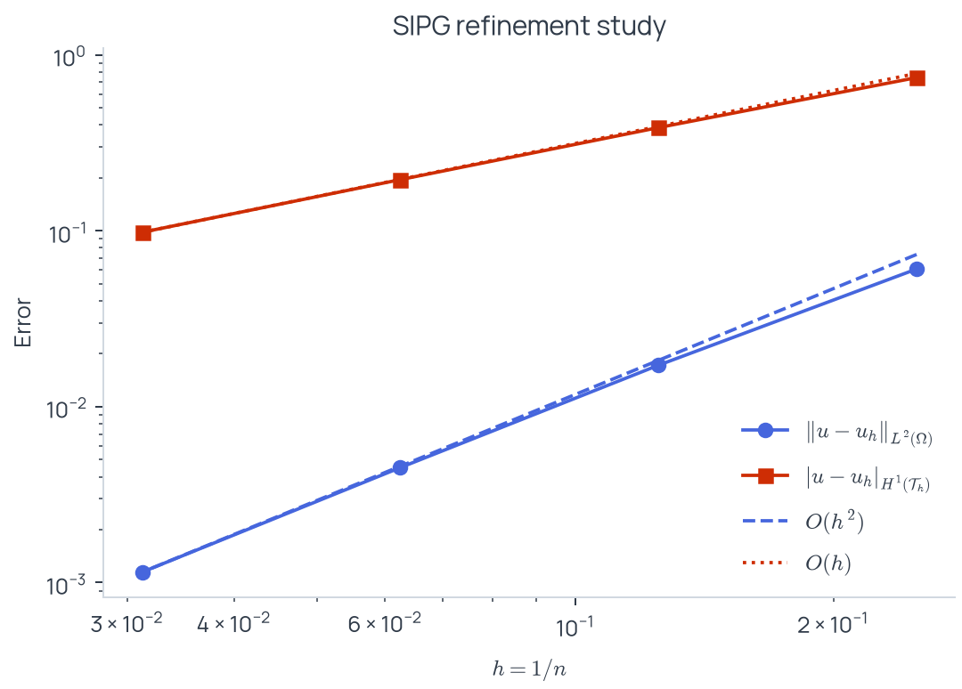
The final refinement gives observed orders approximately 1.97 and 0.99. The unweighted interior jump norm decreases from 0.02846 to 0.001506. The relative matrix-symmetry discrepancy stays below and the relative solution residual below . Positive LDLT pivots are checked at every level.
Preserve separate traces in visualization
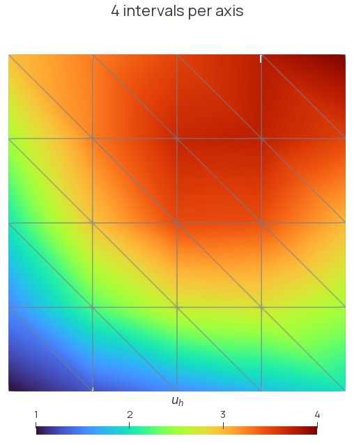
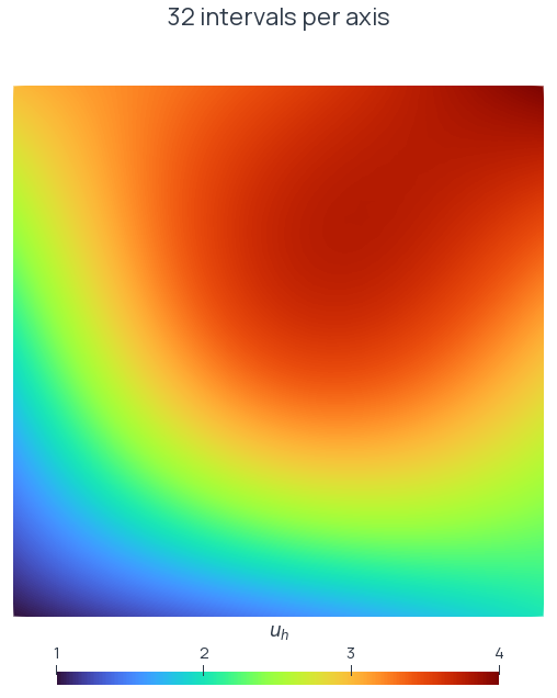
The XDMF output duplicates geometric vertices for each cell so ParaView retains the cell-local values. Open DGCoarse.xdmf or DGPoisson.xdmf, select Apply, then color by u. Keep the original cell-local representation when inspecting jumps.
Build and run
Build DGPoisson and run it in a scratch directory. It executes the patch test and all four refinement levels serially, writes DGConvergence.csv and exports the coarse and finest smooth-case fields. It returns EXIT_FAILURE if factorization, patch accuracy, symmetry, residual, decreasing jumps or the required refinement ratios fail.
Complete source code contains the assembly, numerical checks and visualization export.