Shape optimization of a cantilever

Shows how to optimize the shape of a cantilever.

Introduction

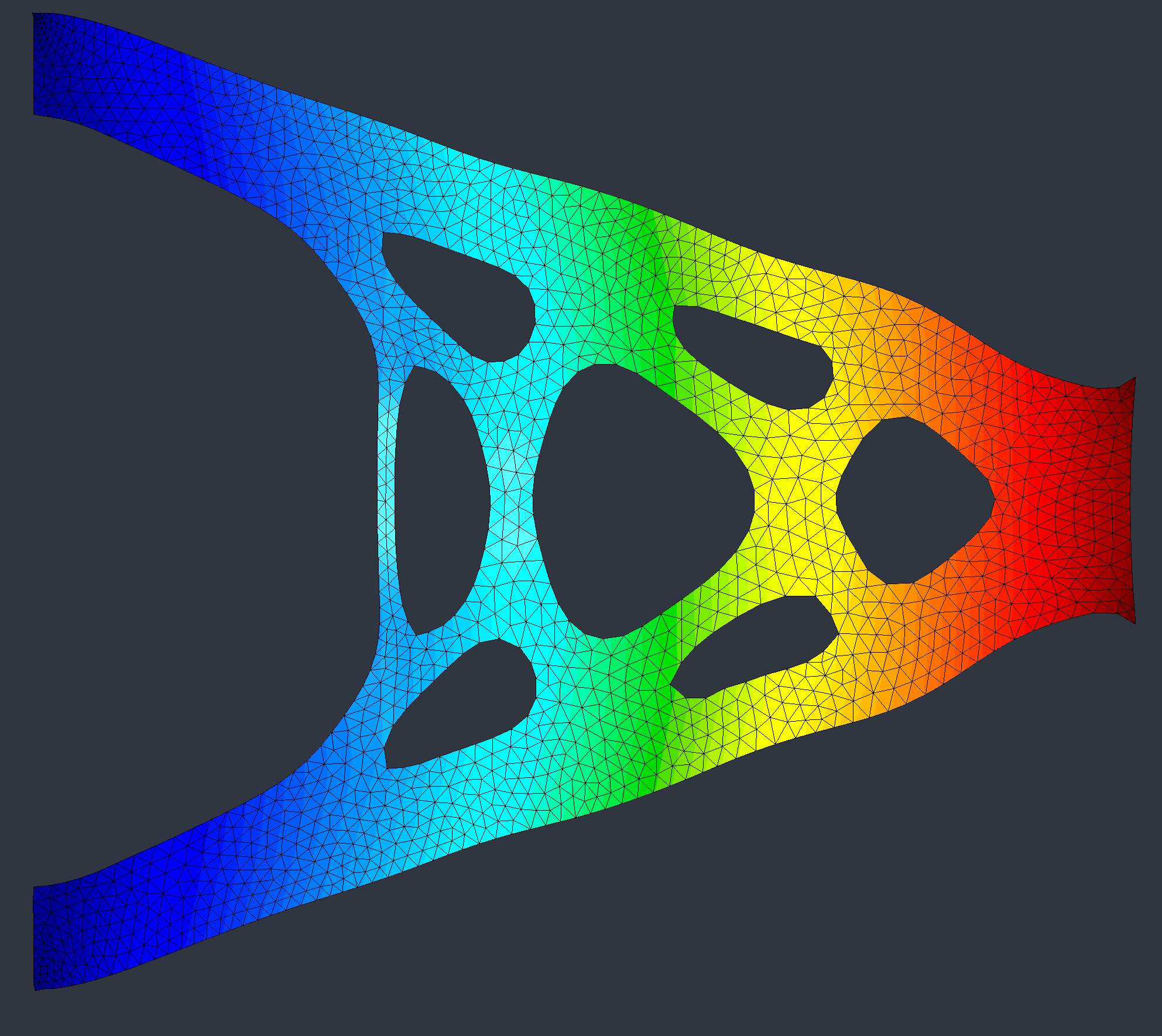
This example performs boundary-variation shape optimization of a 2D cantilever beam. The goal is to find a shape that minimizes the structural compliance (i.e. maximizes stiffness) subject to a volume constraint:

where solves the linearized elasticity system on and is a Lagrange multiplier penalizing the volume.

Problem Setup

Includes

We need the core Rodin modules plus the linear-elasticity helper and the MMG remesher:

#include <Rodin/Solver.h>
#include <Rodin/Geometry.h>
#include <Rodin/Assembly.h>
#include <Rodin/Variational.h>
#include <Rodin/LinearElasticity.h>
#include <Rodin/MMG.h>

using namespace Rodin;
using namespace Rodin::Geometry;
using namespace Rodin::Variational;

Parameters

The boundary is decomposed into three parts:

: traction-free (the shape boundary to be optimized)
: clamped (homogeneous Dirichlet)
: loaded (Neumann, downward force)

static constexpr Geometry::Attribute Gamma0 = 1; // Traction-free boundary
static constexpr Geometry::Attribute GammaD = 2; // Clamped (Dirichlet)
static constexpr Geometry::Attribute GammaN = 3; // Loaded (Neumann)

// Lamé coefficients for the material
static constexpr Real mu     = 0.3846;
static constexpr Real lambda = 0.5769;

// Optimization parameters
static constexpr size_t maxIt = 50;         // Max iterations
static constexpr Real hmax   = 0.1;         // Mesh size (max)
static constexpr Real hmin   = 0.1 * hmax;  // Mesh size (min)
static constexpr Real ell    = 5.0;         // Volume penalty
static constexpr Real alpha  = 4 * hmax;    // Regularization

Loading the Mesh

The initial cantilever mesh is loaded from an MFEM file using the MMG::Mesh class, which extends Mesh with remeshing capabilities:

MMG::Mesh Omega;
Omega.load(meshFile, IO::FileFormat::MFEM);

Optimization Loop

Each iteration consists of four steps:

Solve the state equation (linearized elasticity)
Compute the shape gradient via the Hilbert extension-regularization
Move the mesh along the descent direction
Remesh the deformed domain with MMG

Step 1 — State Equation

We solve the elasticity problem on the current domain. The LinearElasticityIntegral assembles the bilinear form for the Hooke tensor with Lamé parameters and :

int d = Omega.getSpaceDimension();
P1 sh(Omega);           // Scalar P1 space
P1 vh(Omega, d);        // Vector P1 space (d components)

VectorFunction f{0, -1};  // Downward force

TrialFunction u(vh);
TestFunction  v(vh);
Problem elasticity(u, v);
elasticity = LinearElasticityIntegral(u, v)(lambda, mu)
           - BoundaryIntegral(f, v).over(GammaN)
           + DirichletBC(u, VectorFunction{0, 0}).on(GammaD);
Solver::SparseLU(elasticity).solve();

Step 2 — Shape Gradient

The shape derivative of the compliance is a boundary integral involving the Cauchy stress tensor . We compute a smooth descent direction using the Hilbert extension-regularization method:

TrialFunction g(vh);
TestFunction  w(vh);

// Strain and stress from the state equation
auto e  = 0.5 * (Jacobian(u.getSolution()) + Jacobian(u.getSolution()).T());
auto Ae = 2.0 * mu * e + lambda * Trace(e) * IdentityMatrix(d);

Problem hilbert(g, w);
hilbert = Integral(alpha * Jacobian(g), Jacobian(w))
        + Integral(g, w)
        - BoundaryIntegral(Dot(Ae, e) - ell,
                           Dot(BoundaryNormal(Omega), w)).over(Gamma0)
        + DirichletBC(g, VectorFunction{0, 0}).on({GammaD, GammaN});
Solver::SparseLU(hilbert).solve();

Step 3 — Mesh Displacement

The descent direction is normalized and the mesh is displaced:

GridFunction norm(sh);
norm = Frobenius(dJ);
g.getSolution() *= hmin / norm.max();
Omega.displace(g.getSolution());

Step 4 — Remeshing with MMG

After displacing the mesh, we remesh with the MMG::Optimizer to maintain good element quality:

MMG::Optimizer().setHMax(hmax).setHMin(hmin).optimize(Omega);

Full Source Code

The complete source code is:

SimpleCantilever2D.cpp