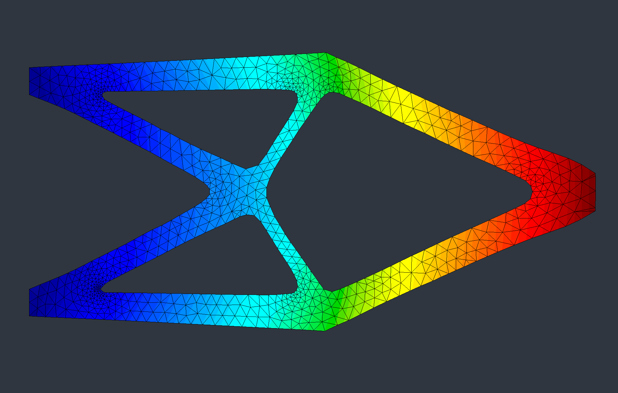
Shape optimization of a cantilever via the level set method

Body-fitted optimization of a cantilever via the level set method.

Introduction

This advanced example combines level-set shape optimization with body-fitted meshing**. Unlike the simple cantilever which only moves the boundary, this algorithm can perform topology changes (create holes, merge components) by advecting a level-set function and recovering the implicit domain at each iteration.

The optimization minimizes compliance subject to a volume constraint:

Problem Setup

Includes

In addition to the standard Rodin modules, we need the Distance module (Eikonal solver) and the Advection module (Lagrangian advection):

#include <Rodin/IO/XDMF.h>
#include <Rodin/Advection/Lagrangian.h>
#include <Rodin/Distance/Eikonal.h>
#include <Rodin/Solver.h>
#include <Rodin/Assembly.h>
#include <Rodin/Geometry.h>
#include <Rodin/Variational.h>
#include <Rodin/LinearElasticity.h>
#include <Rodin/MMG.h>

using namespace Rodin;
using namespace Rodin::Geometry;
using namespace Rodin::Variational;

Parameters

The mesh is partitioned into interior (material present) and exterior (void) regions. The level-set function is positive inside the material and negative outside:

static constexpr Attribute interior = 1, exterior = 2;
static constexpr Attribute Gamma0 = 1, GammaD = 2, GammaN = 3, Gamma = 4;

static constexpr Real mu = 0.3846, lambda = 0.5769;  // Lamé coefficients
static size_t maxIt = 300;                             // Max iterations
static Real hmax = 0.05, hmin = 0.005;                // Mesh sizes
static Real ell = 0.4;                                 // Volume penalty
static Real alpha = 0.1;                               // Regularization

Optimization Loop

Each iteration consists of six steps:

Step 1 — Remesh

At the start of each iteration, we remesh the current domain using MMG::Optimizer:

MMG::Optimizer().setHMax(hmax)
                .setHMin(hmin)
                .setHausdorff(hausd)
                .setAngleDetection(false)
                .optimize(th);

Step 2 — Trim the Mesh

We extract the interior subdomain by trimming the exterior region. The resulting SubMesh inherits boundary attributes from the parent mesh:

SubMesh trimmed = th.trim(exterior);

Step 3 — Solve the State Equation

We solve the elasticity problem on the trimmed (interior) domain:

P1 vhInt(trimmed, d);
TrialFunction u(vhInt);
TestFunction  v(vhInt);

Problem elasticity(u, v);
elasticity = LinearElasticityIntegral(u, v)(lambda, mu)
           - BoundaryIntegral(f, v).over(GammaN)
           + DirichletBC(u, VectorFunction{0, 0}).on(GammaD);
Solver::CG(elasticity).solve();

Step 4 — Shape Gradient

The shape gradient is computed on the full mesh (not trimmed), using traceOf to evaluate quantities from the interior side of the interface :

auto jac = Jacobian(u.getSolution());
jac.traceOf(interior);
auto e  = 0.5 * (jac + jac.T());
auto Ae = 2.0 * mu * e + lambda * Trace(e) * IdentityMatrix(d);
auto n  = FaceNormal(th);
n.traceOf(interior);

TrialFunction g(vh);
TestFunction  w(vh);
Problem hilbert(g, w);
hilbert = Integral(alpha * alpha * Jacobian(g), Jacobian(w))
        + Integral(g, w)
        - FaceIntegral(Dot(Ae, e) - ell, Dot(n, w)).over(Gamma)
        + DirichletBC(g, VectorFunction{0, 0, 0}).on(GammaN);
Solver::CG(hilbert).solve();

Step 5 — Advect the Level Set

The signed distance function is first computed by solving the Eikonal equation** . Then it is advected along the descent direction using a Lagrangian advection scheme:

// Compute signed distance
GridFunction dist(sh);
Distance::Eikonal(dist).setInterior(interior)
                       .setInterface(Gamma)
                       .solve()
                       .sign();

// Advect the level set
TrialFunction advect(sh);
TestFunction  test(sh);
Advection::Lagrangian(advect, test, dist, dJ).step(dt);

Step 6 — Recover the Domain

The new domain is recovered by applying the MMG::LevelSetDiscretizer to the advected level-set function:

th = MMG::LevelSetDiscretizer()
      .split(interior, {interior, exterior})
      .split(exterior, {interior, exterior})
      .setRMC(1e-6)
      .setHMax(hmax).setHMin(hmin).setHausdorff(hausd)
      .setBoundaryReference(Gamma)
      .setBaseReferences(GammaD)
      .discretize(advect.getSolution());

XDMF Output

The XDMF class exports the evolving mesh, distance, and state fields at each iteration for visualization in ParaView:

IO::XDMF xdmf("out/ShapeOptimization");

auto domain = xdmf.grid("domain");
domain.setMesh(th, IO::XDMF::MeshPolicy::Transient);

auto state = xdmf.grid("state");
// ... inside loop:
domain.add("dist", dist, IO::XDMF::Center::Node);
state.setMesh(trimmed, IO::XDMF::MeshPolicy::Transient);
state.add("u", u.getSolution(), IO::XDMF::Center::Node);
xdmf.write(i).flush();

Full Source Code

The complete source code is:

LevelSetCantilever2D.cpp